|
|
|
|
|
In this assignment, I implemented different processes to render an image. In a pathtracing algorithm, I created functions that checks for intersections of primitives with rays in scenes, a data structure to speed up the process of intersections, methods for determining how light travels and bounces around in a scene, and also an overall speedup method for sampling. Through the hours of debugging and waiting for my computer to render images, this project has been the most intensive yet, and I have learned a lot about the interworkings of a scene renderer.
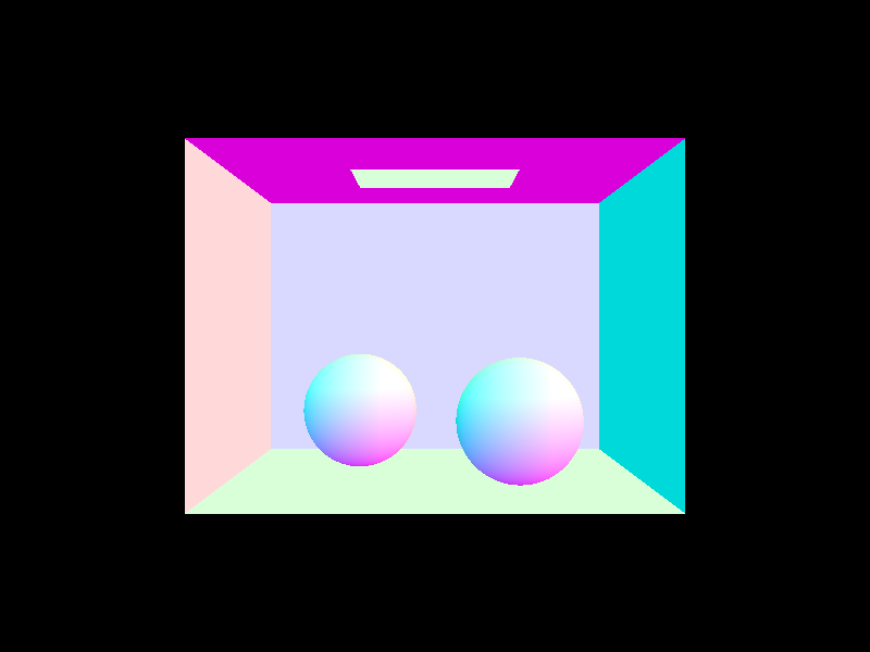
In this part of my project, I implemented a loop in the PathTracer::raytrace_pixel() function that would generate random rays from a specified pixel point. This process requires a conversion from camera space (2D) to world space (3D), which I converted in the Camera::generate_ray() function, and with these random rays, I calculate the irradiance spectrum by summing each individual spectrum and averaging to get an approximate integral of irradiance over the pixel.
Afterwards, we also need to calculate intersection with shapes (such as triangles) to be displayed, so I implemented multiple functions that would check where, if at all, a ray intersected with a designated triangle or sphere. For calculating the intersection of a triangle, I used the Moller Trumbore algorithm, a fast ray-triangle intersection algorithm, to efficiently calculate the position of where an intersection was. This algorithm takes advantage of the barycentric coordinate system within a triangle. Barycentric coordinates require three parameters - w, u, and v - that sum up to 1, so we can replace one of the variables, w, with 1 - u - v (but also making sure that all 3 parameters are between 0 and 1). To solve for the intersection point of the ray with this triangle, we set up the equation between the ray and the triangle:
O + tD = (1 − u − v)A + uB + vC
which can be moved around and simplified to
O - A = −tD + u(B − A) + v(C − A)
We can set up a linear system of equations with this, where
O - A = [-D (B - A) (C - A)]([t u v])^T
To solve the system of linear equations and get unknowns t, u, and v, I applied Cramer's rule. Cramer's rule solves this in terms of the determinant. We solve for the three parameters t, u, and v, where t is the point of intersection for the ray, and u and v give us barycentric coordinates of the intersection on the triangle (we get the w value from 1 - u - v). If the t value we evaluate is between the minimum and maximum values of t for the ray, then we have an intersection, and we re-set the maximum value of the ray to this new t value so that future intersections with this ray will be disregarded.
|
|
|
|
|
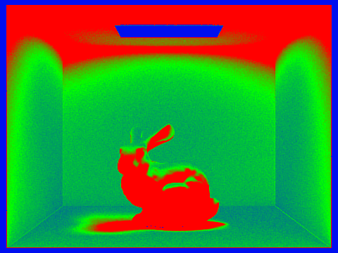
In this section, I implemented a function that would create a bounding volume hierarchy in order to increase efficiency and speed for calculating intersections. A BVH is stored as a tree that holds various geometric shapes, setting these shapes as root nodes of the tree that can be accessed by their bounding boxes.
To implement the BVH, I first collected all of the primitive shapes into one box, keeping track of the bounding volume of the shapes as well as the bounding volume of the center of the shapes. After collecting this data, we check if the number of primitives is less than or equal to the maximum leaf size (if so, we set this as a node that holds all the primitives we have, and we are finished). If not, then we have to split the bounding box so that we would have two different children that potentially hold a smaller number of primitives. The way I implemented this axis split was to find the axis that had the largest dimension (to do this, I got the bbox.extent values and looked for if x, y, or z held the largest value); I split the length of the extent in half, putting elements that had their centroid on one side into a left vector, and the rest of the elements into a right vector. In the case that either the left side or the right side were empty, I would instead split in the middle of the centroid box's extent. This would guarantee that for both sides, I would have at least one primitive. After this finishes, I would recurse down the left and right side using this construct_bvh function on both of the newly created vectors, setting these to be the left and ride side of the current node, and then afterwards returning the current node.
The way we speed up the process of intersections using BVH's is by only traversing those primitives if its bounding box intersects with the ray; this avoids the need to expensively check many primitives that are assured to be a non-intersection. The way we calculate the intersection of a bounding box is by calculating the intersection between the ray and the individual axes - keep in mind we are calculated the axes because we are going to use the axis-aligned box intersection method. To do this, we keep track of the t-values that the ray enters each plane as well as exiting each plane. We pretty much find the maximum t for entrance and minimum t for exit because this is the point where the ray enters the block from all 3 dimensions (or exits the block depending on which t you are looking at). The equation for finding the intersection of a plane and a ray is as follows:
t = ((p - o) * N) / (d * N)
Where p is a point on the plane, o is the origin of the ray, N is a vector orthogonal to the plan going out, d is the direction of the ray, and t is the time of intersection.
If the time of exit is greater than the time of entrance, then we know that the ray intersects with the bounding box. So, the way our intersection function works is that we repeat this process until we get to a leaf node of the BVH. This holds all of the primitives that are in the BVH, so we check to see if the ray intersects with any of these primitives. Since we are doing this to all bounding boxes that are in the way of the ray, then we will be able to find the first primitive that the ray intersects with since we minimize the ray's t value every time we have an intersection with a primitive.
|
|
|
|
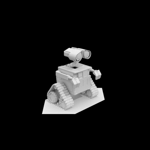
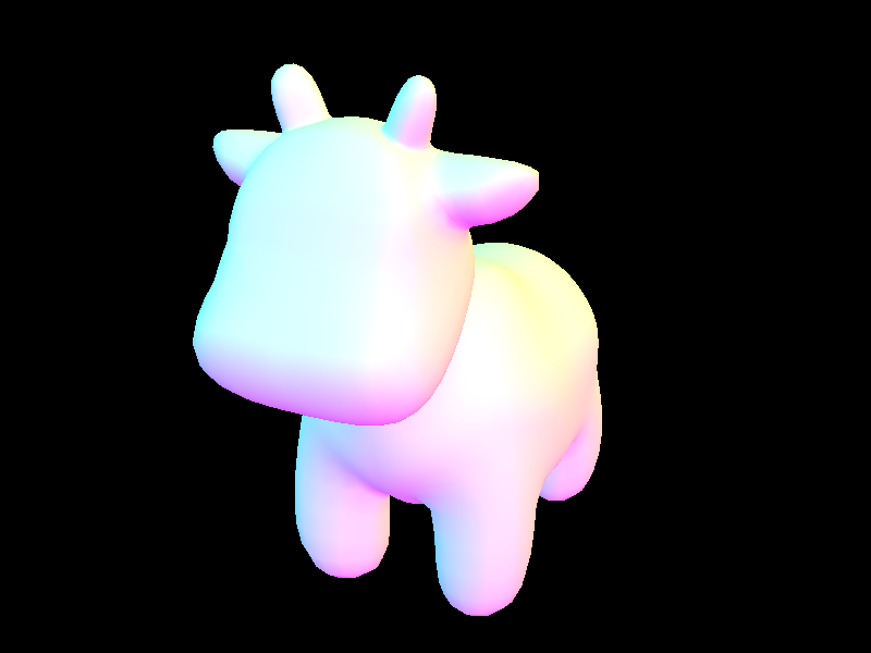
When analyzing the speed of rendering between using BVH's and not using BVH's, having a BVH signiciantly increases the speed. Rendering the cow.dae file without BVH took approximately 5 minutes and 56 seconds, but with BVH took only 0.6265 seconds. When I rendered bunny.dae naively, it took approximately 38 minutes and 45 seconds (using my stopwatch), but rendering with a BVH took 0.5804 seconds (these were done on my personal computer). This is because when we are using bounding boxes, we are reducing the amount of primitives that we are checking for an intersection, which overall speeds the process so that we wouldn't have to check unneccessary parts of the model.
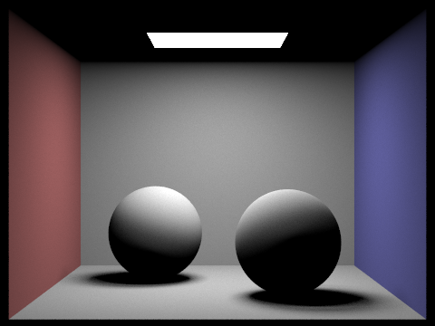
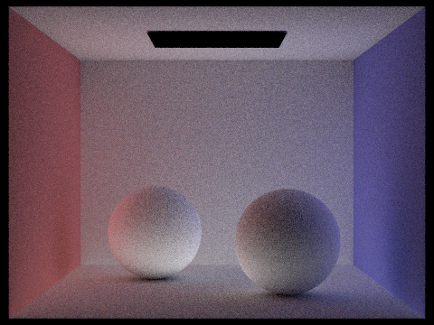
I implemented two methods to estimate direct lighting, which are uniform hemisphere sampling and importance sampling. These functions give us different ways to calculate light hitting a surface and how much is being reflected off, which relies on the BSDF (Bidirectional Scattering Distribution Function) that I implemented in first task of this part.
The basis of uniform hemisphere sampling is to sample random rays that center around the point in question, and accumulate the radiance that hits the point if our ray intersects a light source. My sampling loop iterates for a given number of samples, creating a random ray in each iteration (we get the ray from a simple sample that we convert from local object space to world space, with the origin being the hit point plus a tiny global constant). We then check if this ray intersects with any light source by using our bvh->intersect method, and if it does, then we calculate the radiance of that intersecting point. Before we add this radiance to the total, we need to also convert it into irradiance; to do that, we multiply radiance by the BSDF of the input and output vectors, as well as the cosine of the incoming vector. We also need to divide by the number of samples in order to have our sum become the average irradiance, and also weight our result by the pdf.
Importance sampling is slightly similar to uniform sampling. In this method, I instead sample over all of the light sources in the scene. Within these samples, we have to again iterate through a certain number of samples. If it were the case that our current light source is a delta light, then we would only have to sample once because all the samples would be the exact same. If not, then we would have to iterate through the length of ns_area_light as our number of samples instead. Once we start the for loop, we do operations similar to what was performed for uniform hemisphere sampling - we get a random sample, create a ray, and check for intersections - but with slight changes. We get a sample from the light source instead of a vector pointing out of the hit point. I also check if the z coordinate in the sampled vector is negative because it would reduce the amount of intersections I would need to check (if z were negative, then the sampled vector point lies behind the surface so it wouldn't be spotted). Also, instead of adding samples if they intersected, we add them if they don't intersect with anything. This is because we want the ray to reach to the source without being disrupted by other primitives in the way.
|
|
|

|
Noise levels in soft shadows with various light rays and 1 sample per pixel using light sampling:
|

|
|

|
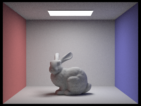
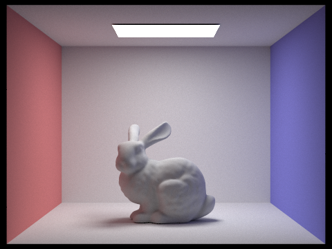
The noise in the shadows of the bunny became less apparent as we increased the amount of light rays in the scene, and it became more obvious to figure out the shape of the shadow with the increased amount of light rays.
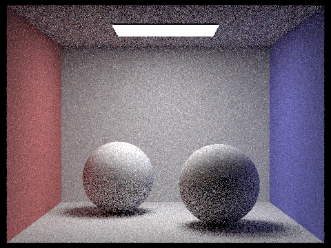
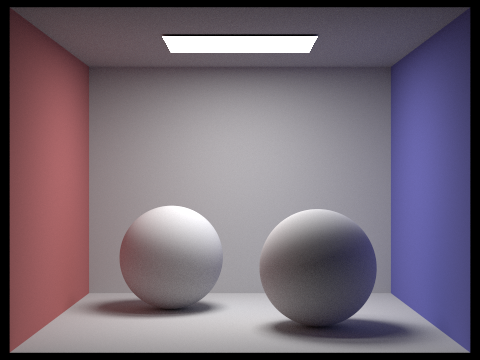
Overall, the images that were illuminated using importance sampling could efficiently have less noise than the images using uniform hemisphere sampling. When we use more samples with uniform hemisphere sampling, we get less noise and appear to have similar results to importance sampling, but this comes at the cost of performance, because the amount of time it takes to render an images slows down significantly. In the case of the CBbunny.dae file (on the hive computers), it took 23.47 seconds to render using 8 light rays and 16 samples per pixel, and it took 373.66 seconds seconds to render using 32 light rays and 64 samples per pixel, but improving the resulting image. However, our importance sampling method yields a far better picture with 32 light rays and 64 samples per pixel but takes 296.54 seconds, which is shorter than the time it took to render using uniform hemisphere sampling, as well as equally decent pictures using 64 light rays and 1 pixel which only took 0.21 seconds to render.
Indirect lighting is created from rays bouncing off of surfaces. In this section we implemented a process that would allow for indirect illumination, by creating functions that return light resulting from various bounces of light. For a zero bounce light, I just return isect.bsdf->get_emission(), which is no emission unless we are on a light source. For a one bounce light, we just use the functions from part 3 because one bounce is the same as direct illumination. However, when we need to calculate a light that bounces at least once, it gets a little more complicated and we have to use recursion. Because we are going to be recursively calling at_least_one_bounce_radiance, we need to have some sort of indicator of where we should terminate. The way we do this is by creating a Russian roulette method that would terminate the ray at a random time given a probability of termination - my termination probability was 0.3 (probability of not terminating a ray was 0.7). Also the name of this function (at_least_one_bounce_radiance) implies that we have to recurse at least once, so what I did to resolve that was to set ray depth equal to max_ray_depth whenever a ray was created, and in the function, I state that we recurse for sure if ray depth equals max_ray_depth, but also decrement ray depth when I go into that recursion step. Once the recursive steps terminate, we collect the radiance and convert it into outgoing radiance (similar to part 3), scaling by the BSDF and cosine, but also dividing by the pdf as well as 1 - termination probability, which in our case is 0.7.

|
|
|
|
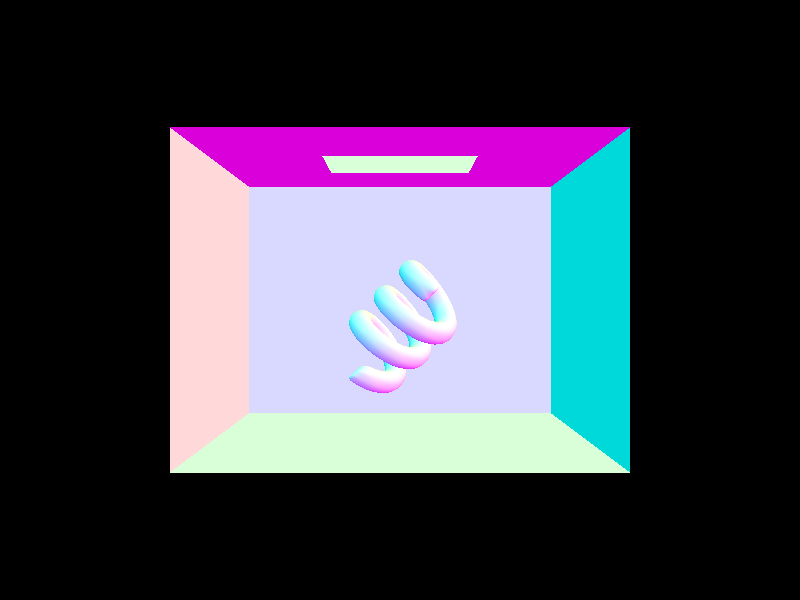
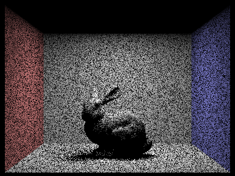
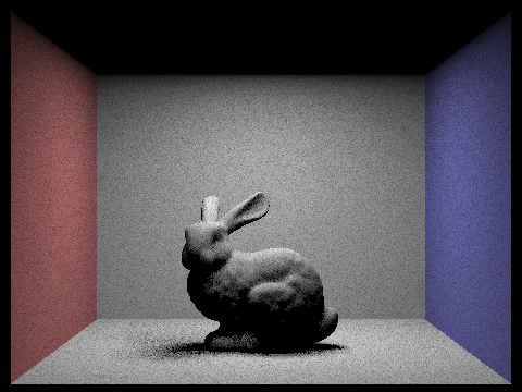
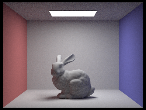
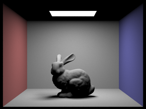
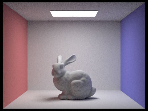
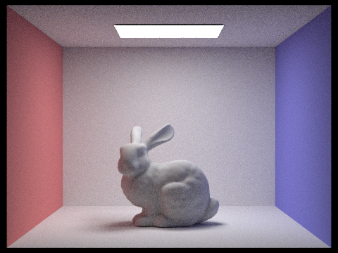
Now we will compare rendered views by changing max_ray_depth. We see that with a max ray depth of 0, there is no light reflected and the only light we see is from the light souce. A depth of 1 shows the first bounce of light, and in greater max depths we see that the bouncing of light causes a slight overall brightness, as well as shadows that are less dark.
|
|
|
|
|
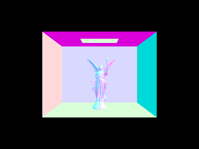
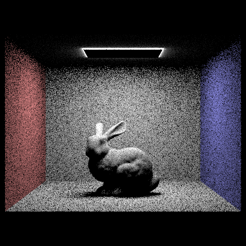
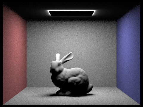
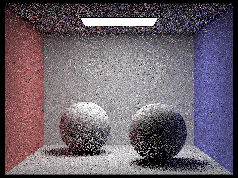
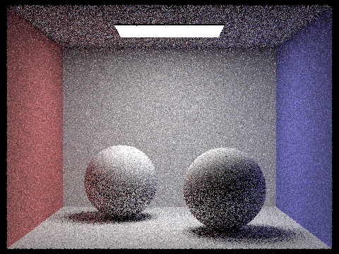
Now we will compare rendered views by changing sample-per-pixel rates. We see that if we increase the amount of samples per pixel, there is less noise in the overall picture.
|
|
|

|

|

|
|
Adaptive sampling is a way of altering the amount of samples so that we would not require excessive samples on a certain pixel. Thus, we can get rid of excess noise faster if we can tell whether or not the pixel converges at a lower rate. To implement this, I used an adaptive sampling algorithm and made some changes to raytrace_pixel(), a function I implemented in part 1 of the project.
The adaptive sampling algorithm terminates differently for each pixel based on some statistics. I need to calculate the mean and variance of the illuminace, so every time I get a sample, I add its illuminance to s1 (s1/n is the mean where n is the number of samples), and add its illuminance squared to s2 (the variance is (1 / (n - 1)) * (s2 - ((s1 * s1) / n)))
So, with the sample mean m and variance o, we want to reach a 95% confidence of having an average illuminance between m - I amd m + I, where I is represented as
I = 1.96 * sqrt(o) / sqrt(n)
which is the formula from determining a confidence interval given a mean and standard deviation. So, if it were the case that
I <= maxTolerance * m
If this equation is satisfied, then we can stop performing additional samples because we know that the pixel has converged. So, I stop sampling more rays at this point and I return the average spectrum, keeping into account that the number of samples is now just the amount that I stopped at. I also put this number of samples into a vector that keeps track of the sample count for all points on the picture, so that we get another picture which is the sample rate of every pixel due to adaptive sampling.
|
|