|
|
|
|
|
In this project, I continued where I left off with ray tracing in the previous project. I implemented new BSDF materials such as mirror and glass (calculating reflection and refraction), as well as surfaces with microfacets such as copper and gold. I implemented ways to use environment maps and infinite environment lights in part 3, which is useful when not having a background in your rendering scene. I also created a depth of field simulator that would focus on certain parts of the image given a specified lens radius and focal distance. In the last part, I used a shader program, GLSL, to speed up rendering and learned how to calculate different shading methods relying on vertex and fragment shaders. This was a very extensive project, and even though it was difficult to figure out what to do in each part, I am very satisfied with my end results and can confidently say I have a very decent rendering machine.
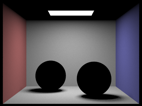
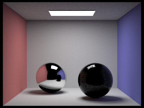
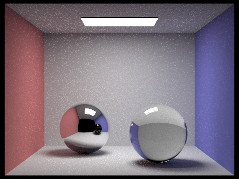
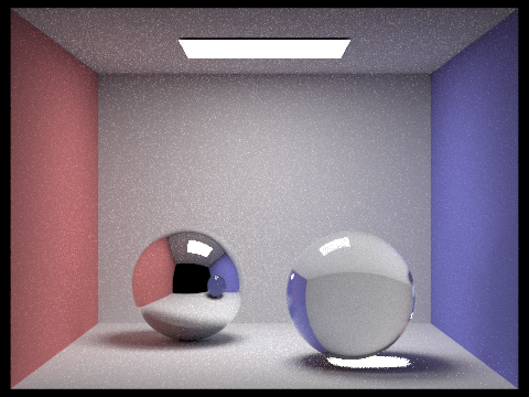
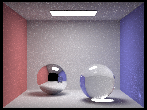
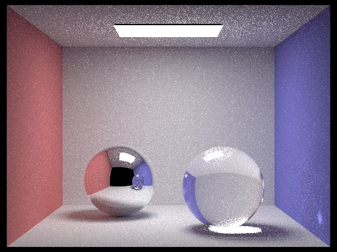
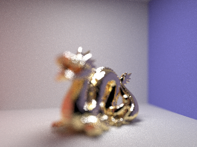
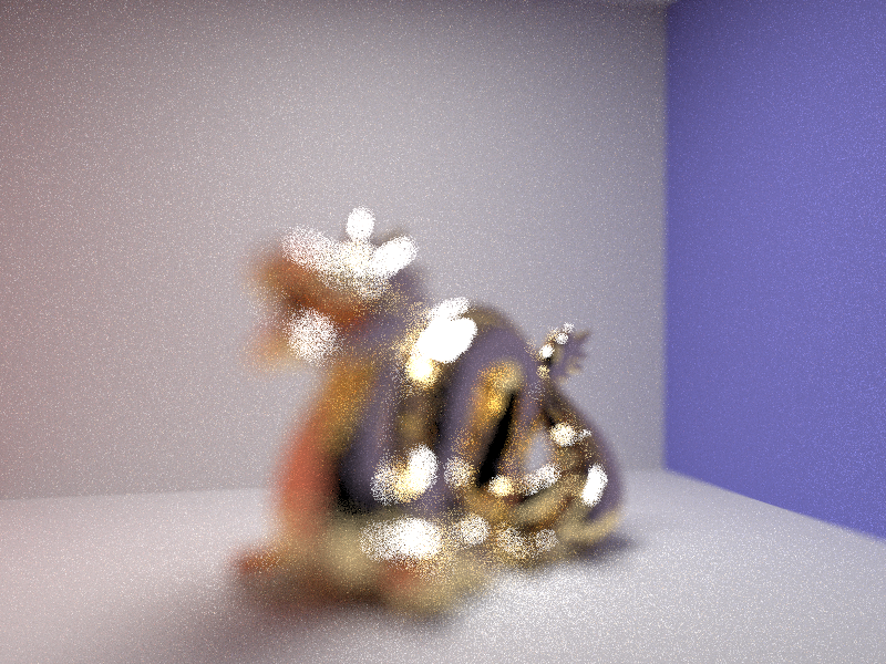
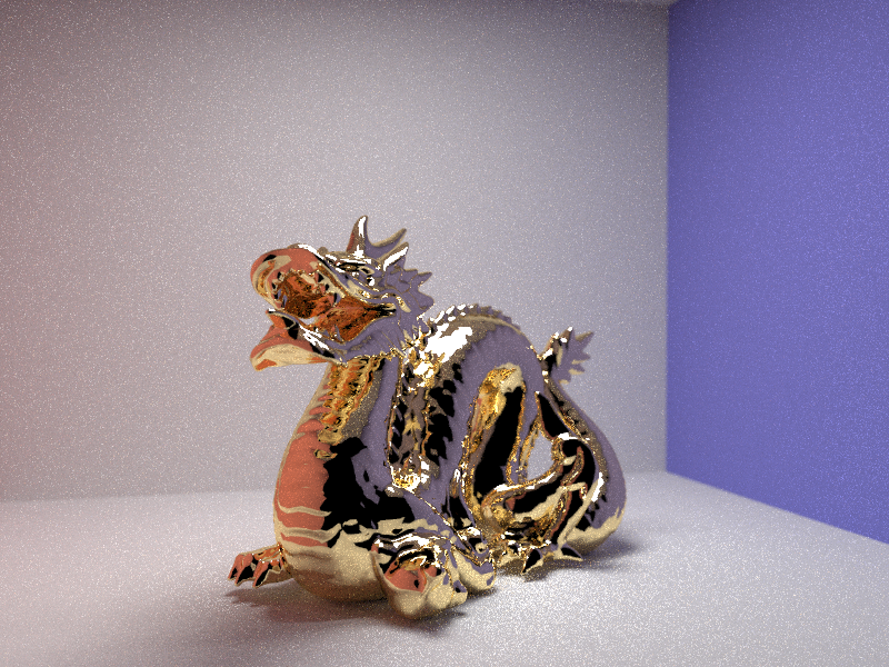
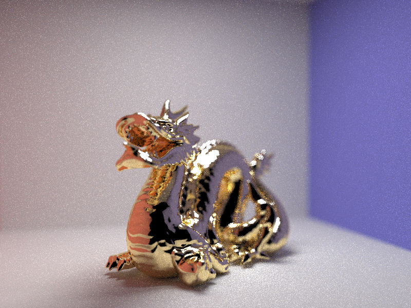
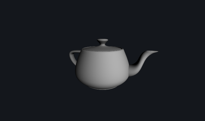
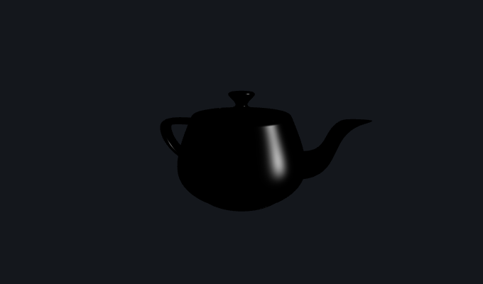
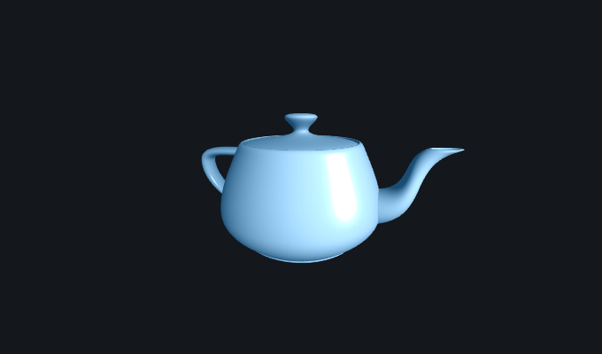
In the first part of the project, I made functions that allowed for reflection and refraction on surfaces, which is used for the mirror and glass material. The following images show the process of rays bouncing through the scene of CBspheres.dae, starting from 0 bounces and going to 100 bounces.
|
|
|
|
|
|
|
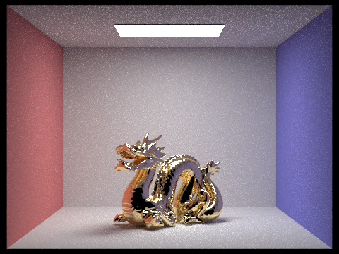
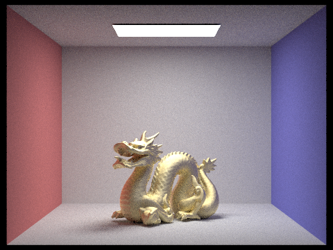
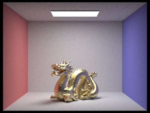
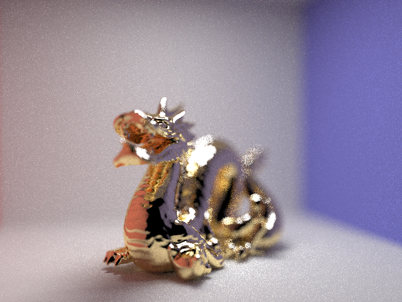
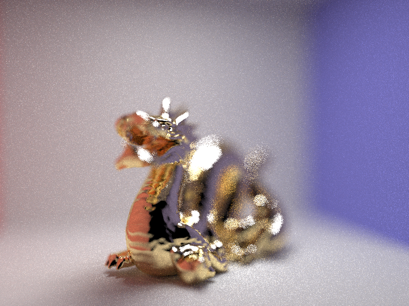
In part 2, I implemented the microfacet model, which is basically a texture for the material that determines how smooth or rough the surface is, which in turn determines how much light is reflected and spread out over a certain area of the model. I also had to implement functions that would compute the Fresnel term, Shadow-Masking term, and the Normal Distribution Function in order to piece together the specific microfacet BRDF.
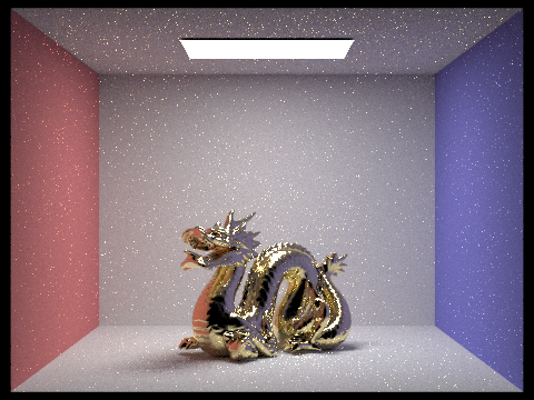
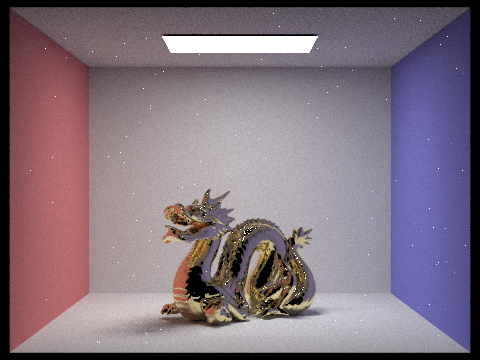
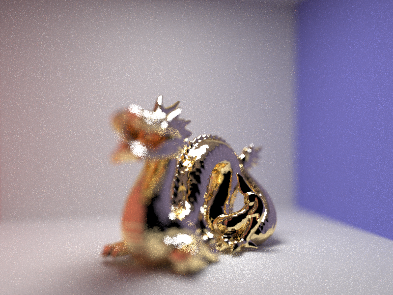
With the following section, I tested on CB_dragon_microfacet_au.dae with various alpha values to see the amount of reflection that varied between the different values. A high alpha rate (0.5) represents a more diffuse material, meaning that it is rougher and the light spreads around the surface more. A low alpha rate (0.005) would represent a glossy material, appearing much more smooth and reflective on the model's surroundings. In between, we see a mixture of both, where the image is still slightly fuzzy while having some reflectance.
|
|
|
|
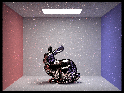
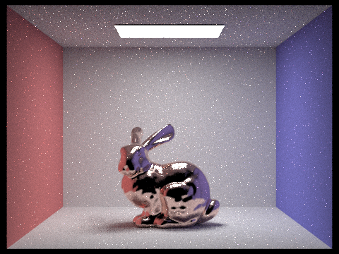
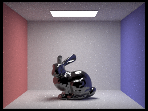
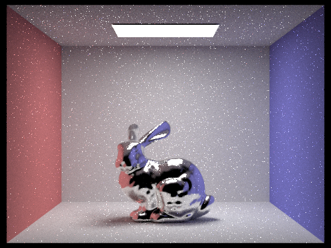
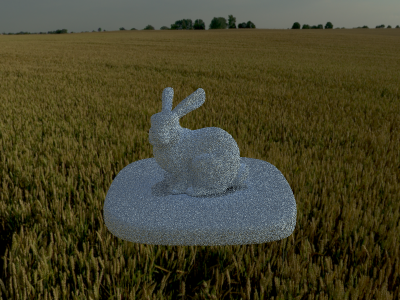
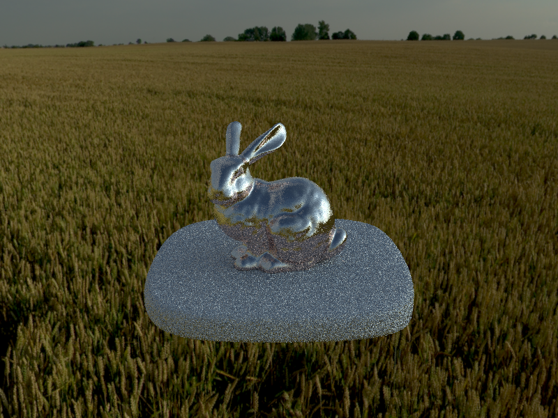
The two images below are renderings of the copper bunny using two different techniques: cosine hemisphere sampling and importance sampling. The default code given beforehand was cosine hemisphere sampling, which is more inefficient because the scene requires a lot more samples before it converges. I compare the two using the same constraints - 64 samples per pixel, 1 sample per light, and a maximum of 5 bounces. We see that my implemented importance sampling method renders a picture with a better defined material than the rendering using basic cosine hemisphere sampling.
|
|
I altered the CBbunny dae file to produce a bunny that was made out of the material Carbon as well as a bunny made out of the material Sodium. I used the website refractiveindex.info in order to find the eta and k values of the material at specific wavelengths 614 nm (red), 549 nm (green), and 466 nm (blue).
|
|
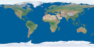
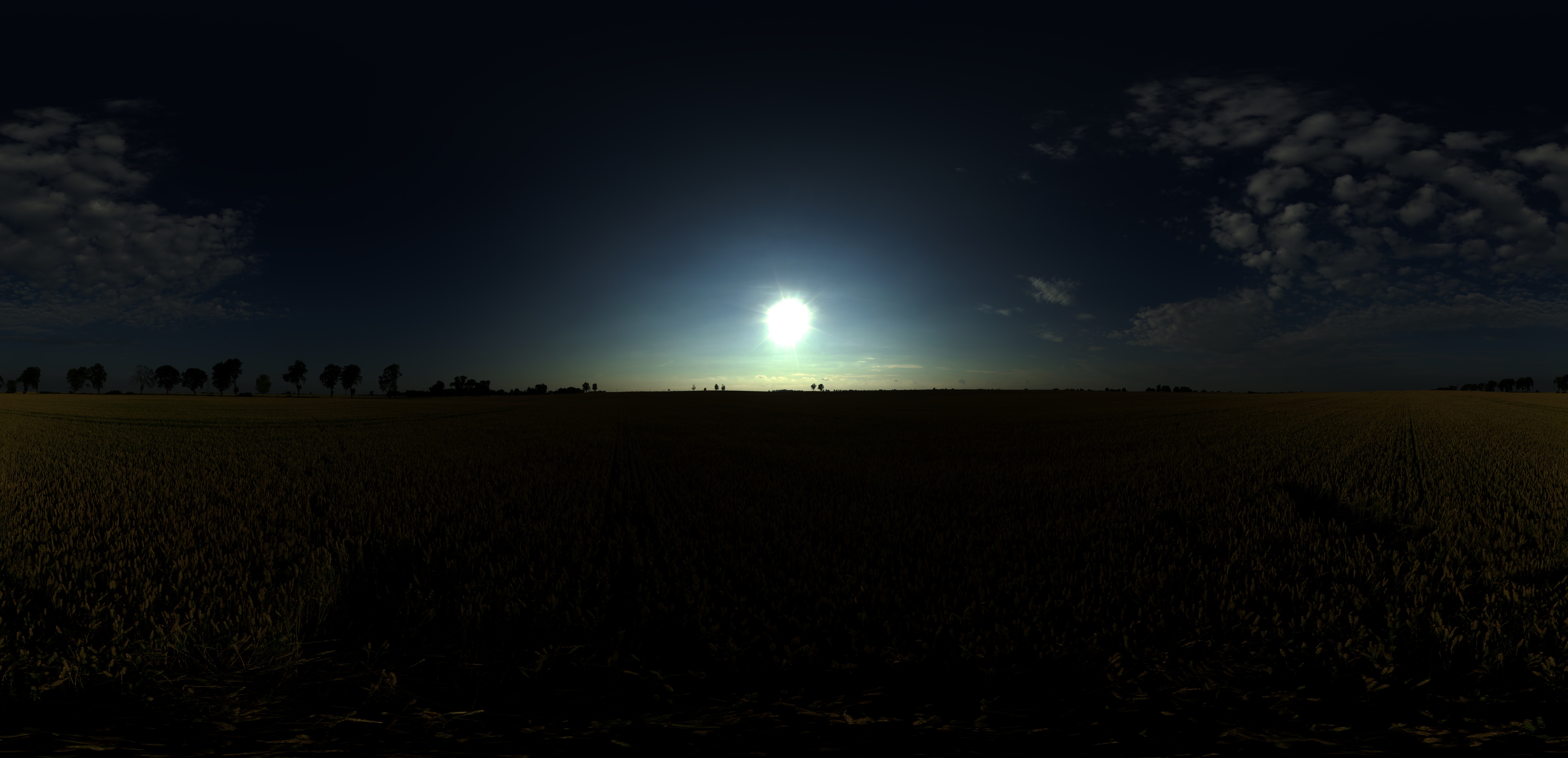
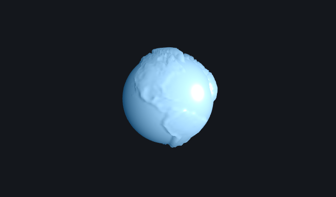
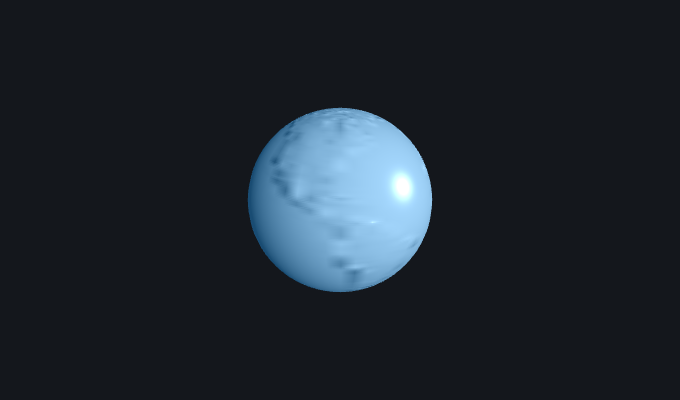
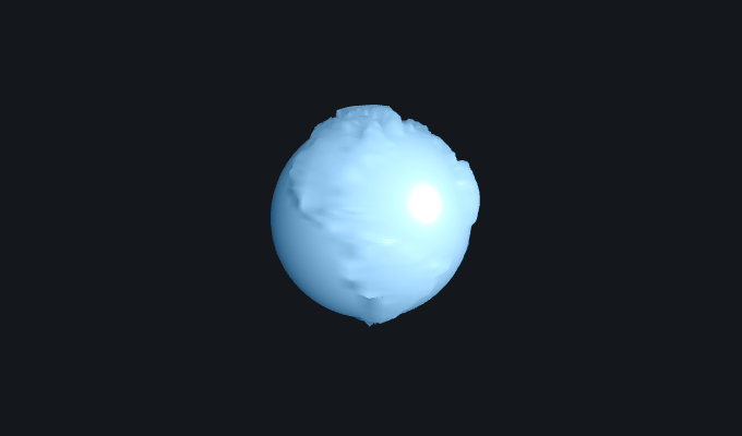
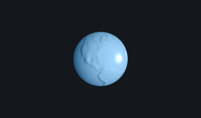
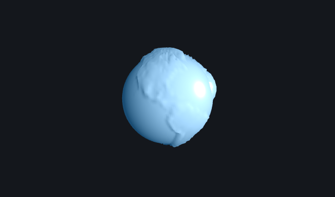
In this section, I created functions that would accomodate for scenes that had no light source. Because of this, the new type of light source that would make up the scene is an infinite environment light. We use this environment map only when there is no intersection in the scene with the ray (no walls to hit basically) and if there actually does exist an environment map for us to use. I implemented both uniform sampling and importance sampling techniques to render the environment map lights.
The environment map I am using is field.exr (see below for picture of field).
| |
|
Comparing bunny_unlit.dae uniform sampling versus importance sampling. The render with uniform sampling appears to be more grainy, and the render with importance sampling has a better defined shadow. This was done with 4 samples per pixel, 64 samples per light, and a max ray depth of 5.

|
|
Comparing bunny_microfacet_cu_unlit.dae uniform sampling versus importance sampling. Similar to the normal unlit file, the render with uniform sampling appears to be more grainy with a less defined shadow. This was done with 4 samples per pixel, 64 samples per light, and a max ray depth of 5.
|

|
One last note for my part 3 - it may seem like the fields for uniform sampling look darker than the fields for importance sampling, but I assure you that is not the case (it is an optical illusion)! If you place the images back to back, for instance having both images in separate tabs and switching between them, you would be able to tell that the fields are the same.
Before implementing this part, my images were clear in focus no matter how far or close the object was, which represented a pin-hole camera model. In this part, I simulated a depth of field as if I were generating rays through a thin lens. This essentially makes objects look more focused only if they are on the plane of focus, which is determined by a specified lens radius and focal distance.
These four images are a "focus stack" of the dragon microfacet BSDF, which is just the same scene but focused at different depths of the scene. This was done with 64 samples per pixel, 4 samples per light, and a max ray depth of 8. The aperture size was left at a constant 0.0883883.
|
|
|
|
These four images are of the dragon microfacet BSDF, focused at the same depth, but with different aperture sizes. This was done with 64 samples per pixel, 4 samples per light, and a max ray depth of 8. The depth was left at a constant 1.7. It appears that a smaller aperture size correlated with a larger depth of field.
|
|
|
|
Refer to this link to see gl in the works (my gl page)!
This part of the project was quite different from the previous parts. I used GLSL, a C-ish programming language to compute shading on objects. This allows for an accelerated render compared to the previous parts which took more than a couple minutes to render (GLSL computes in parallel on the GPU, a Graphics Processing Unit designated for creating images quickly). We perform shading on vertices and fragments by computing the color of each individual piece (whether it be a vertex or a fragment).
With the accelerated shader program, I was able to implement Blinn-Phong Shading, which is a technique that takes three different shading models - ambient shading (lighting), diffuse shading (reflection), and specular shading (highlights) - and combines them to create a reflection model. This allows us to generate an image that is less computationally-expensive, while still maintaining decent shading overall.

|
|
|
|
My third task was to implement texture mapping, which takes a given uv image and maps it to an object given uv coordinates. The following is the result of my implementation.
|

|
In the next part, I implemented bump mapping and displacement mapping, which simulated depth and actual roughness in the object based on lighting. When comparing the two textures, it is noticeable that bump mapping doesn't actually create physical depth in the object (as we rotate the object), however, displacement actually creates depth which we can see in the image.

|
|
When altering the vertical and horizontal components to see how mesh coarseness would be affected, I noticed that decreasing the number of horizontal components made both object seem more stretched out horizontally, and decreasing the number of vertical components seemed to make it appear stretched out vertically. This is similar to how sampling less points leads to images that are less accurate and less clear.
|
|
|
|
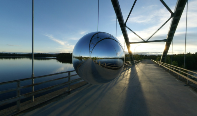
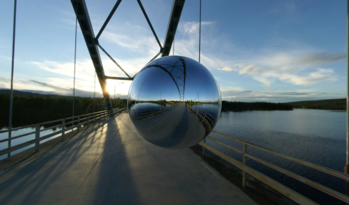
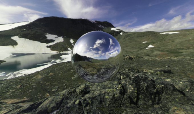
For my custom shader, I implemented an object that would appear to reflect the scene onto itself, like a ball made out of mirror material! Frustrating parts of implementing this was trying to figure out how GLSL worked, and how to add a cube background to the scene. In the end, I am very proud of the work I did to figure out the basics of node.js and how to render scenes through a shader program. I got these cube background scenes from Emil Persson's site.
|
|